
Technical material
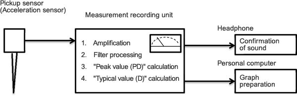
The pickup sensor of the groundwater aeration sound measuring device GAS-03 senses the sound (vibration) transmitted underground as acceleration (m/s2) and converts the magnitude of the acceleration into voltage (mV). In the measurement recording unit, the converted voltage signal is amplified and then the low frequency and high frequency signals are erased with the filter, thereby making it easier to distinguish the groundwater aeration sound by hearing it. Also, in the calculation processing, primary processing and secondary processing are performed to express the loudness of groundwater aeration sound in numerical values so that the intensity of sound can be judged, and the loudness is displayed on the LCD panel in numerical values, and at the same time it is indicated on the level meter (Fig. 1).
Overview of data processing
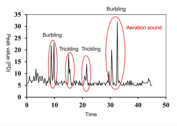
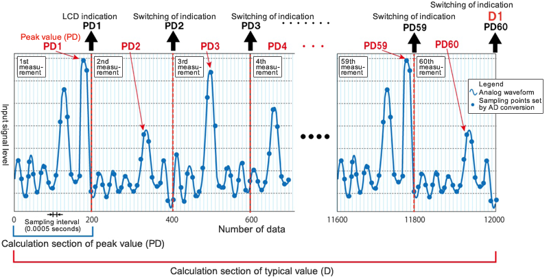
Fig. 2 shows waveforms after processing groundwater aeration sound. The groundwater aeration sound has a peak as shown in Fig. 2 when burbling sounds are given off. In the calculation processing, many peak values of such burbling sounds are collected, and their average is obtained to calculate the typical value (D) of the groundwater aeration sound. In the calculation processing, in order to calculate the typical value (D), 2 steps of processing consisting of primary processing and secondary processing are performed. Their details are explained below.
[1] Primary processing (collection of the peak value (PD) of unprocessed data)
In the primary processing, the input data are sampled once every 0.5 msec (2 KHz), and the maximum value is collected at set intervals (number of samples). The maximum value obtained here is called the "peak value (PD)" and this processing is done 60 times to calculate 60 values: "peak value: PD1" - "peak value: PD60." Also, the number of samples can be set to a value in the range from 100 to 500 at intervals of 50 on the setting screen of "Setting/Sampling."
Fig. 3 shows an example of collection of peak values (PDs) from the input data when the number of samples is set to 200 (the original graph has 200 sample points per 1 time of measurement, but the number of points has been omitted to make the graph easier to see).
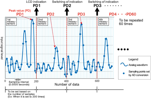
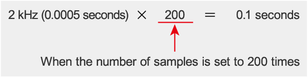
Also, when the number of samples is set to 200 times, the maximum value is to be obtained from 200 data that have been obtained in 0.1 seconds as shown in the following equation.
When capturing the source of sound to be measured (aeration sound of water, etc. in the case of water flowing underground), settings can be made so that more desired sounds will be captured by changing the number of samples (in the case of water flowing underground, the quantity of aeration sound varies with the type of geology).
Although the existing setting of the number of samples is 200 times, if the number of desired sources of sound is small, the desired sources of sound are likely to be captured by setting a greater number of samples (longer time of measurement) and if the number of desired sources of sound is great, by setting a smaller number of samples (shorter time of measurement). However, if a longer time of measurement is set, noise is likely to get in due to movement during measurement, etc. Also, since the time for calculating the peak value (PD) varies with the setting value of the number of samples, attention needs to be paid to this fact when comparing results obtained under different setting conditions.
[2] Secondary processing (calculation of the typical value "D")
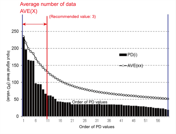
In the secondary processing, the greatest value is obtained among the 60 "peak values (PDs)" from the primary processing or multiple "peak values (PDs)" obtained in descending order from the greatest value are averaged. (The number of values can be changed by settings.)
The greatest value or average thus obtained is called the "typical value (D)" (Fig. 4).
The method of calculation of the typical value (D) can be selected from the following 2 patterns: A and B.
A. Detect the greatest value among the 60 peak values (PDs) and use it as the typical value (D).
Typical value (D) = Peak value (PD) max
B. From the 60 peak values (PDs), pick out a set number of peak values (PDs) in descending order from the greatest value, and obtain the average of such values, and use it as the typical value (D).
In the average number of data: AVE(X), set how many peak values (PDs) obtained in descending order from the greatest value will be averaged.
Typical value (D) = (Peak value 1 (PD1) + Peak value 2 (PD2) + ... + Peak value (X) (PD(X)))/N(X)
Whether the calculation method "A" is used or the calculation method "B" is used can be changed by settings.
When the method of "B" has been selected, the number of maximum values to be picked out can be set within the range of 2 - 60 values by the setting for the average number of data (Fig. 5 shows a graph of 60 peak values that have been rearranged in descending order).
Also, as the average number of data increases, the typical value (D) becomes smaller.
Method of conversion of the peak value (PD) and typical value (D) into acceleration units
The peak value (PD) and typical value (D) are index values. The loudness of groundwater aeration sound can be compared by using the values as they are, but it is also possible to obtain acceleration (m/s2) from these index values.
Fig. 6 shows the relations between the peak value (PD), typical value (D) and acceleration when AMP has been changed between 1 and 10.
The peak value (PD) and typical value (D) change within the range of 0 - 999, whereas acceleration increases steeply like a cubic function.
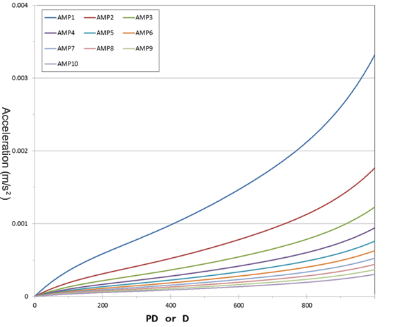
The relations shown in Fig. 6 between the index values: "peak value (PD)," "typical value (D)" and acceleration (m/s2) can be represented by Equation [1].
G=(1.37561×10⁻¹⁷×X5 - 3.3382×10⁻¹⁴×X4 + 3.26003×10⁻¹¹×X3-1.44833×10⁻⁸×X2 + 4.81626×10⁻⁶×X)/ Ki [1]
G: Acceleration (m/s2)
X: Index value (peak value (PD) or typical value (D))
Ki: Coefficient determined by the setting of AMP(i) (see Table 1), i: Setting value of AMP (1 - 10)
| AMP(i) | 1 | 2 | 3 | 4 | 5 | 6 | 7 | 8 | 9 | 10 |
|---|---|---|---|---|---|---|---|---|---|---|
| Rate of amplification | 0.0917 | 0.1724 | 0.2579 | 0.3226 | 0.400 | 0.4839 | 0.5885 | 0.6897 | 0.8257 | 1.0 |
| Coefficient Ki | 1.00 | 1.88 | 2.70 | 3.52 | 4.36 | 5.27 | 6.31 | 7.52 | 9.00 | 10.90 |
· An example of conversion into acceleration
An example of conversion from the peak value (PD) into acceleration is shown below.
When the conditions of measurement AMP=5, and the measured value, i.e. peak value (PD)=156:
Since X=156 and Ki=4.36, acceleration G (156) becomes as follows
Acceleration G (156)
=(1.37561×10-17×1565-3.3382×10-14×1564+3.26003×10-11×1563
-1.44833×10-8×1562+4.81626×10-6×156)/4.36
=(1.27092×10⁻⁶-1.97739×10⁻⁵+1.23764×10⁻⁴
-3.52466×10⁻⁴+7.51337×10⁻⁴)/4.36
= 0.000504/4.36
= 0.000116
When AMP=5 and the measured peak value (PD) is 156, the acceleration becomes: 0.000116 (m/s2).
Time required to obtain the peak value (PD) and typical value (D)
The typical value (D) is a value obtained by averaging the top n peak values (PDs) in arbitrary time, and is determined by the setting for the average number of data AVE(n). The arbitrary time is determined by the setting value of the number of samples as shown in Table 2.
Now, let us consider the time TPD for obtaining PD in the case of the number of samples = 200, and the time TD for obtaining D. By accumulating 200 data that have been measured at a sampling cycle of 0.5 msec (2000 Hz), and the maximum value obtained from them becomes PD, and hence
TPD = 0.5 msec (2000 Hz)×200 pieces= 0.1 (sec)
and PD becomes the maximum value in 0.1 seconds.
By accumulating 60 PDs that have been obtained in this period of 0.1 seconds, and the average of the top n pieces becomes the D value, and hence
TD = 0.1 sec × 60 pieces = 6 (sec)
and it follows that D is obtained in 6 seconds.
The time TD for obtaining the typical value (D) varies with the number of samples (50 - 500) as shown in Table 2.
As described above, the typical value (D) becomes the average of the top n pieces in the 60 peak values (PDs) in the arbitrary time shown in Table 1.
| Number of samples | 50 | 100 | 150 | 200 | 250 | 300 | 350 | 400 | 450 | 500 |
|---|---|---|---|---|---|---|---|---|---|---|
| TPD | 0.025 | 0.05 | 0.075 | 0.1 | 0.125 | 0.15 | 0.175 | 0.2 | 0.225 | 0.25 |
| TD | 1.5 | 3 | 4.5 | 6 | 7.5 | 9 | 10.5 | 12 | 13.5 | 15 |
* Number of samples: Number of data and setting values required for obtaining the peak value (PD)
* TPD: Time required for obtaining the peak value (PD) (sec)
* TD: Time required for obtaining the typical value (D) (sec)